Did you Miss me? PyCon IL 2023

Today I talked about working with missing data at PyCon IL. We started with a bit of theory about mechanisms of missing data –

  • MCAR – The fact that the data are missing is independent of the observed and unobserved data.
  • MAR – The fact that the data are missing is systematically related to the observed but not the unobserved data.
  • MNAR – The fact that the data are missing is systematically related to the unobserved data.

And deep-dived into an almost real-world example that utilizes the Python ecosystem – pandas, scikit-learn, and missingno.

My slides are available here and my code is here.

3 related posts I wrote about working with missing data in Python –

Pandas fillna vs scikit-learn SimpleImputer

Missing data is prevalent in real-world data and can be missing for various reasons. Gladly, both pandas and scikit-learn several imputation tools to deal with it. Pandas offers a basic yet powerful interface for univariate imputations using fillna and more advanced functionality using interpolate. scikit-learn offers both SimpleImputer for univariate imputations and KNNImputer and IterativeImputer for multivariate imputations. In this post, we will focus on fillna and SimpleImputer functionality and compare them.

Basic Functionality

SimpleImputer offers four strategies to fill in the nan values – mean, median, most_frequet, and constant.

import numpy as np
import pandas as pd
from sklearn.impute import SimpleImputer

df = pd.DataFrame(
    [[7, 2, np.nan], [4, np.nan, 6], [10, 5, 9]])
imp_mean = SimpleImputer(strategy='mean')
pd.DataFrame(imp_mean.fit_transform(df))

output –

      0    1    2
0   7.0  2.0  7.5
1   4.0  3.5  6.0
2  10.0  5.0  9.0

Can we achieve the same with pandas? Yes!

df.fillna(df.mean())

Want to impute with the most frequent value?

Asuume – df = pd.DataFrame(['a', 'a', 'b', np.nan])

With SimpleImputer

imp_mode = SimpleImputer(
    strategy='most_frequent')
pd.DataFrame(
  
  imp_mode.fit_transform(df))

With fillna

df.fillna(df.mode()[0])

And the output of both –

   0
0  a
1  a
2  b
3  a

Different Strategies

Want to apply different strategies for different columns? using scikit-learn you will need several imputers, one per each strategy. Using fillna you can pass a dictionary, for example –

df = pd.DataFrame(
    [[7, 2, np.nan], [4, np.nan, 6], [10, 5, 9]])
df.fillna({1: 10000, 2: df[2].mean()})
    0        1    2
0   7      2.0  7.5
1   4  10000.0  6.0
2  10      5.0  9.0

Advanced Usage

Want to impute values drawn from a normal distribution, no brainer –

mean = 5
scale = 2
df = pd.DataFrame(
    [[7, 2, np.nan], [4, np.nan, 6], [10, 5, 9]])
df.fillna(
    pd.DataFrame(
        (np.random.normal(mean, scale, df.shape))
    0         1         2
0   7  2.000000  3.857513
1   4  5.407452  6.000000
2  10  5.000000  9.000000

Missing indicator

Using SimpleImputer, one can add indicator columns that obtain 1 if the original column was missing, and 0 otherwise. This can also be done using MissingIndicator

df = pd.DataFrame(
    [[7, 2, np.nan], [4, np.nan, 6], [10, 5, 9]])
mean_imp = SimpleImputer(strategy='mean', add_indicator=True)
mean_imp.fit_transform(df)
pd.DataFrame(mean_imp.fit_transform(df))
      0    1    2    3    4
0   7.0  2.0  7.5  0.0  1.0
1   4.0  3.5  6.0  1.0  0.0
2  10.0  5.0  9.0  0.0  0.0

Note that a missing column (i.e., columns 3 and 4 in the example above) corresponds only to columns with missing values. Therefore there is no missing indicator column corresponding to the column 0. If you are converting back and forth to pandas dataframes you should note this nuance.

Another nuance to note when working with SimpleImputer is that columns that contain only missing values are dropped by default –

df =  pd.DataFrame(
    [[7, 2, np.nan, np.nan], [4, np.nan, 6, np.nan],
    [10, 5, 9, np.nan]])
mean_imp = SimpleImputer(strategy='mean')
pd.DataFrame(mean_imp.fit_transform(df))
      0    1    2
0   7.0  2.0  7.5
1   4.0  3.5  6.0
2  10.0  5.0  9.0

This behavior is controllable using setting keep_empty_features=True. While it is manageable, tracing columns might be challenging –

mean_imp = SimpleImputer(
    strategy='mean',
    keep_empty_features=True,
    add_indicator=True)
pd.DataFrame(mean_imp.fit_transform(df))
      0    1    2    3    4    5    6
0   7.0  2.0  7.5  0.0  0.0  1.0  1.0
1   4.0  3.5  6.0  0.0  1.0  0.0  1.0
2  10.0  5.0  9.0  0.0  0.0  0.0  1.0

There is an elegant way to achieve similar behavior in pandas –

df = pd.DataFrame(
    [[7, 2, np.nan, np.nan], [4, np.nan, 6, np.nan],
     [10, 5, 9, np.nan]])
pd.concat(
    [df.fillna(df.mean()), 
     df.isnull().astype(int).add_suffix("_ind")], axis=1)
    0    1    2   3  0_ind  1_ind  2_ind  3_ind
0   7  2.0  7.5 NaN      0      0      1      1
1   4  3.5  6.0 NaN      0      1      0      1
2  10  5.0  9.0 NaN      0      0      0      1

Working with dates

Want to work with dates and fill several columns with different types? No problem with pandas –

df = pd.DataFrame(
    {"date": [
        datetime(2023, 6, 20), np.nan,
        datetime(2023, 6, 18), datetime(2023, 6, 16)],
     "values": [np.nan, 1, 3, np.nan]})
df.fillna(df.mean())

Before –

        date  values
0 2023-06-20     NaN
1        NaT     1.0
2 2023-06-18     3.0
3 2023-06-16     NaN

After –

        date  values
0 2023-06-20     2.0
1 2023-06-18     1.0
2 2023-06-18     3.0
3 2023-06-16     2.0

Working with dates is an advantage that fillna has over SimpleImputer.

Backward and forward filling

So far, we treated the records and their order as independent. That is, we could have shuffled the records and that would not affect the expected imputed value. However, there are cases, for example, when representing time series when the order matters and we would like to impute based on later values (backfill) or earlier values (forward fill). This is done by setting the method property.

df = pd.DataFrame(
    [[7, 2, np.nan], [4, np.nan, 6],
     [10, np.nan, 9], [np.nan, 5, 10]])
df.fillna(method='bfill')
      0    1     2
0   7.0  2.0   6.0
1   4.0  5.0   6.0
2  10.0  5.0   9.0
3   NaN  5.0  10.0

One can also limit the number of consecutive values which are imputed –

df.fillna(method='bfill', limit=1)
      0    1     2
0   7.0  2.0   6.0
1   4.0  NaN   6.0
2  10.0  5.0   9.0
3   NaN  5.0  10.0

Note that when using bfill or ffill and moreover, when specifying limit to value other than None it is possible that not all the values would be imputed.

For me, that’s a killer feature of fillna comparing to SimpleImputer

Treat Infinite values as na

Setting pd.options.mode.use_inf_as_na = True will treat infinite values (i.e. np.inf, np.INF, np.NINF) values as missing values, for example –

df = pd.DataFrame([1, 2, np.inf, np.nan])
df.fillna(1000)

pd.options.mode.use_inf_as_na = False

     0
0  1.0
1  2.0
2  inf
3  1000.0

pd.options.mode.use_inf_as_na = True

     0
0  1.0
1  2.0
2  1000.0
3  1000.0

Note that inf and na are not treated the same for other use cases, e.g. – df[0].value_counts(dropna=False)

0
1.0    1
2.0    1
NaN    1
NaN    1

Summary

Both pandas and scikit-learn offer a basic functionality to deal with missing values. Assuming you are working with pandas Dataframe, pandas fillna functionality can achieve everything SimpleImputer can do and more – working with dates, back and forward fill, etc. Additionally, there are some edge cases and specific behaviors to pay attention to when choosing what to use. For example when using bfill or ffill method some values may not be imputed if there are the last ones or first ones respectively.

Exploratory Data Analysis Course – Draft

Last week I gave an extended version of my talk about box plots in Noa Cohen‘s Introduction to Data Science class at Azrieli College of Engineering Jerusalem. Slides can be found here.

The students are 3rd and 4th-year students, and some will become data scientists and analysts. Their questions and comments and my experience with junior data analysts made me understand that a big gap they have in purchasing those positions and performing well is doing EDA – exploratory data analysis. This reminded me of the missing semester of your CS education – skills that are needed and sometimes perceived as common knowledge in the industry but are not taught or talked about in academia. 

“Exploratory Data Analysis (EDA) is the crucial process of using summary statistics and graphical representations to perform preliminary investigations on data in order to uncover patterns, detect anomalies, test hypotheses, and verify assumptions.” (see more here). EDA plays an important role in everyday life of anyone working with data – data scientists, analysts, and data engineers. It is often also relevant for managers and developers to solve the issues they face better and more efficiently and to communicate their work and findings.

I started rolling in my head how would a EDA course would look like –

Module 1 – Back to basics (3 weeks)

  1. Data types of variables, types of data
  2. Basic statistics and probability, correlation
  3. Anscombe’s quartet
  4. Hands on lab – Python basics (pandas, numpy, etc.)

Module 2 – Data visualization (3 weeks)

  1. Basic data visualizations and when to use them – pie chart, bar charts, etc.
  2. Theory of graphical representation (e.g Grammar of graphics or something more up-to-date about human perception)
  3. Beautiful lies – graphical caveats (e.g. box plot)
  4. Hands-on lab – python data visualization packages (matplotlib, plotly, etc.).

Module 3 – Working with non-tabular data (4 weeks)

  1. Data exploration on textual data
  2. Time series – anomaly detection
  3. Data exploration on images

Module 4 – Missing data (2 weeks)

  1. Missing data patterns
  2. Imputations
  • Hands-on lab – a combination of missing data \ non-tabular data

Extras if time allows-

  1. Working with unbalanced data
  2. Algorithmic fairness and biases
  3. Data exploration on graph data

I’m very open to exploring and discussing this topic more. Feel free to reach out – twitterLinkedIn

pandas read_csv and missing values

I read Domino Lab post about “Data Exploration with Pandas Profiler and D-Tale” where they load diagnostic mammograms used in the diagnostic of breast cancer from UCI website. Instead of missiing values the data contains ?. When reading the data using pandas read_csv function naively interpret the value as string value and change the column type to be object instead of float in this case.

In the post mentioned above the authors dealt with the issue in the following way –

masses = masses.replace('?', np.NAN)
masses.loc[:,names[:-1]] = masses.loc[:,names[:-1]].apply(pd.to_numeric)

That is, they first replaced the ? values in all the columns with np.NAN and then convert all the columns to numeric. Let’s call this method the manual method.

If we know the know the non default missing values in advance, can we do something better? The answer is yes!

See code here

Use na_values parameter

df = pd.read_csv(url, names=names, na_values=["?"])

na_values parameter can get scalar, string, list-like or dict parameters. If you pass a scalar, string or list-like parameter all columns are treated the same way. If you pass dict you can specify different set of NaN values per column.

The advantage of this method over the manual method is that you don’t need to convert the columns after replacing the nan values. In the manual method the column types are specified (in the given case they are all numeric), if there are multiple columns types you need to know it and specify it in advance.

Side note – likewise, for non trivial boolean values you can use true_values and false_values parameters.

Use converters parameter

df = pd.read_csv(url, names=names, converters={"BI-RADS": lambda x: x if x!="?" else np.NAN})

This is usually used to convert values of specific columns. If you would like to convert values in all the columns in the same way this is not the preferred method since you will have to add an entry for each column and if new column is added you won’t take care of it by default (this can be both advantage and disadvantage). However, for other use-cases, converters can help with more complex conversions.

Note that the result here is different then the result in the other methods since we only converted the values in one column.

Conclusion

Pandas provides several ways to deal with non-trivial missing values. If you know the non-trivial value in advance you are good to go and na_values is most likely the best way to go.

Performance wise (time) all methods perform roughly the same for the given dataset but that can change as a function on the dataset size (columns and rows), row types, number of non-trivial missing values.

On top of it, make reading documentation your superpower. It can use your tools smarter and more efficient and it can save you a lot of time.

See pandas read_csv documentation here

5 tips for using Pandas

Recently, I worked closely with Pandas and found out a few things that are might common knowledge but were new to me and helped me write more efficient code in less time.


1. Don’t drop the na

Count the number of unique values including Na values.

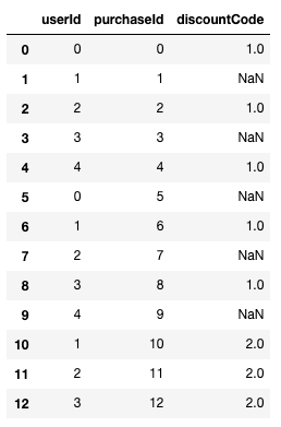
Consider the following pandas DataFrame –

df = pd.DataFrame({"userId": list(range(5))*2 +[1, 2, 3],
                   "purchaseId": range(13),
                   "discountCode": [1, None]*5 + [2, 2, 2]})

Result

If I want to count the discount codes by type I might use –  df['discountCode'].value_counts() which yields – 

1.0    5
2.0    3

This will miss the purchases without discount codes. If I also care about those, I should do –

df['discountCode'].value_counts(dropna=False)

which yields –

NaN    5
1.0    5
2.0    3

This is also relevant for nuniqiue. For example, if I want to count the number of unique discount codes a user used – df.groupby("userId").agg(count=("discountCode", lambda x: x.nunique(dropna=False)))

See more here – https://pandas.pydata.org/pandas-docs/stable/reference/api/pandas.DataFrame.nunique.html

2. Margin on Row \ columns  only

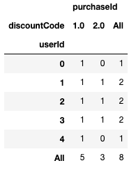
 Following the above example, assume you want to know for each discount code which users used it and for each user which discount code she used. Additionally you want to know has many unique discount codes each user used and how many unique users used each code, you can use pivot table with margins argument –

df.pivot_table(index="userId", columns="discountCode",
               aggfunc="nunique", fill_value=0,
               margins=True)

Result –

It would be nice to have the option to get margins only for rows or only for columns. The dropna option does not act as expected – the na values are taken into account in the aggregation function but not added as a column or an index in the resulted Dataframe.

3. plotly backend


Pandas plotting capabilities is nice but you can go one step further and use plotly very easy by setting plotly as pandas plotting backend.  Just add the following line after importing pandas (no need to import plotly, you do need to install it) –

pd.options.plotting.backend = "plotly"

Note that plotly still don’t support all pandas plotting options (e.g subplots, hexbins) but I believe it will improve in the future. 


See more here – https://plotly.com/python/pandas-backend/


4. Categorical dtype and qcut

Categorical variables are common – e.g., gender, race, part of day, etc. They can be ordered (e.g part of day) or unordered (e.g gender). Using categorical data type one can validate data values better and compare them in case they are ordered (see user guide here). qcut allows us to customize binning for discrete and categorical data.

See documentation here and the post the caught my attention about it here – https://medium.com/datadriveninvestor/5-cool-advanced-pandas-techniques-for-data-scientists-c5a59ae0625d

5. tqdm integration


tqdm is a progress bar that wraps any Python iterable, you can also use to follow the progress of pandas apply functionality using progress_apply instead of apply (you need to initialize tqdm before by doing tqdm.pandas()).

See more here – https://github.com/tqdm/tqdm#pandas-integration

5 interesting things (04/12/2020)

How to set compensation using commonsense principles – yet another artwork by Erik Bernhardsson. I like his analytics approach and the way he models his ideas. His manifest regarding compensation systems (Good/bad compensation systems) is brilliant. I believe most of us agree with him while he put it into words. His modeling has some drawbacks that he is aware of. For example, assuming certainty in employee productivity, almost perfect knowledge of the market. Yet, it is totally worth your time.

https://erikbern.com/2020/06/08/how-to-set-compensation-using-commonsense-principles.html

7 Over Sampling techniques to handle Imbalanced Data – imbalanced data is a common real world scenario, specifically in healthcare where most of the patients don’t have a certain condition one is looking for. Over-sampling is a method to handle imbalanced data, this post describes several techniques to handle it. Interestingly, at least in this specific example, most of the techniques do not bring significant improvement. I would therefore compare several techniques and won’t just try one of them. 
https://towardsdatascience.com/7-over-sampling-techniques-to-handle-imbalanced-data-ec51c8db349f

This post uses a the following package which I didn’t know before (it would be great if it could become part of scikit-learn) – https://imbalanced-learn.readthedocs.io/en/stable/index.html

It would be nice to see a similar post fo downsampling techniques.


Python’s do’s and don’t do – very nicely and written with good examples – 
https://towardsdatascience.com/10-quick-and-clean-coding-hacks-in-python-1ccb16aa571b

Every Complex DataFrame Manipulation, Explained & Visualized Intuitively – can’t remember how pandas function work? great, you are not alone. You can use this guide to quickly remind you how melt, explode, pivot and others work.
https://medium.com/analytics-vidhya/every-dataframe-manipulation-explained-visualized-intuitively-dbeea7a5529e

Causal Inference that’s not A/B Testing: Theory & Practical Guide – Causality is often overlooked in the industry. Many times you developed a model that is “good enough” and move on. However, this might increase bias and lead to unfavourable results. This post suggests a hands-on approach to causality accompanied by code samples.

https://towardsdatascience.com/causal-inference-thats-not-a-b-testing-theory-practical-guide-f3c824ac9ed2